Math Breakdown
Introduction
This section explains in full detail how our solver calculates equilibrium concentrations in a system involving the binding of two proteins:
Protein A (or A) and Protein B
(or B), and the competitive inhibition by an inhibitor
(or I). We will cover every algebraic derivation step from the mass-action formulation through to the final
numerical solution. The goal is to allow a reader to follow every reasoning step, even if the process is lengthy.
Species color template
Theoretical Background: Mass-Action Equilibrium
The basis of our model is the mass-action law, which states that the rate of a chemical reaction is proportional to the
product of the reactants' concentrations. For the reaction where Protein A
binds Protein B:
\[
A + B \rightleftharpoons AB \quad \text{with} \quad K_{d1} = \frac{[A]_{\text{free}} \cdot [B]_{\text{free}}}{[AB]}
\]
Here, \(K_{d1}\) is the dissociation constant that quantifies the binding affinity between A
and B.
Deriving the Binding Equation for A-B Complex
Mass Balance: The total amounts of A and B
can be divided between the free and the bound forms:
- \([A]_{\text{tot}} = [A]_{\text{free}} + [AB]\)
- \([B]_{\text{tot}} = [B]_{\text{free}} + [AB]\)
We express the free concentrations as:
\[
[A]_{\text{free}} = [A]_{\text{tot}} - [AB], \qquad [B]_{\text{free}} = [B]_{\text{tot}} - [AB]
\]
By substituting these into the equilibrium (mass-action) equation we have:
\[
K_{d1} = \frac{([A]_{\text{tot}} - [AB]) ([B]_{\text{tot}} - [AB])}{[AB]}
\]
Multiplying both sides by [AB] gives:
\[
K_{d1}[AB] = ([A]_{\text{tot}} - [AB]) ([B]_{\text{tot}} - [AB])
\]
Expanding the right-hand side:
\[
K_{d1}[AB] = [A]_{\text{tot}}[B]_{\text{tot}} - [A]_{\text{tot}}[AB] - [B]_{\text{tot}}[AB] + [AB]^2
\]
Rearranging terms yields the quadratic equation:
\[
[AB]^2 - ([A]_{\text{tot}} + [B]_{\text{tot}} + K_{d1})[AB] + [A]_{\text{tot}}[B]_{\text{tot}} = 0
\]
The quadratic formula gives the exact concentration of the complex:
\[
[AB] = \frac{([A]_{\text{tot}} + [B]_{\text{tot}} + K_{d1}) \pm \sqrt{([A]_{\text{tot}} + [B]_{\text{tot}} + K_{d1})^2 - 4[A]_{\text{tot}}[B]_{\text{tot}}}}{2}
\]
Since the concentration must be positive, we choose the solution with the negative square root.
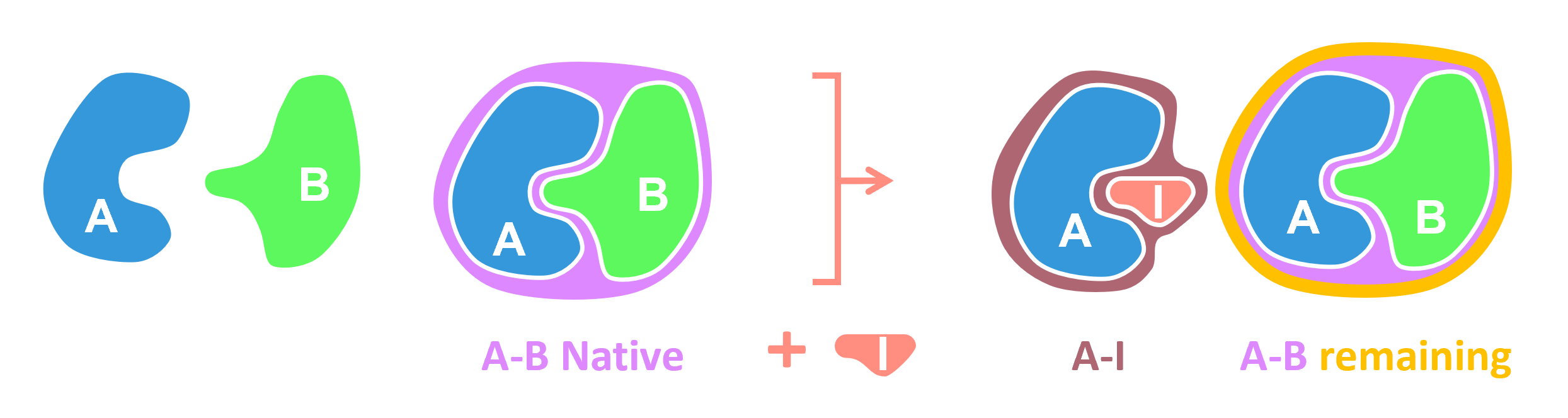
Accounting for Competitive Inhibition
When an inhibitor (I) is introduced, Protein A
can bind both Protein B and the inhibitor.
Hence, we also consider the equilibrium:
\[
A + I \rightleftharpoons AI \quad \text{with} \quad K_{d2} = \frac{[A]_{\text{free}} \cdot [I]_{\text{free}}}{[AI]}
\]
New Mass Balances: The total concentrations become:
- \([A]_{\text{tot}} = [A]_{\text{free}} + [AB] + [AI]\)
- \([B]_{\text{tot}} = [B]_{\text{free}} + [AB]\)
- \([I]_{\text{tot}} = [I]_{\text{free}} + [AI]\)
Expressing the free concentrations:
\[
[A]_{\text{free}} = [A]_{\text{tot}} - [AB] - [AI]
\]
\[
[B]_{\text{free}} = [B]_{\text{tot}} - [AB]
\]
\[
[I]_{\text{free}} = [I]_{\text{tot}} - [AI]
\]
Inserting these into the equilibrium equations results in:
\[
K_{d1} = \frac{([A]_{\text{tot}} - [AB] - [AI]) ([B]_{\text{tot}} - [AB])}{[AB]}
\]
\[
K_{d2} = \frac{([A]_{\text{tot}} - [AB] - [AI]) ([I]_{\text{tot}} - [AI])}{[AI]}
\]
Defining \(x = [AB]\) and \(y = [AI]\), we obtain the coupled equations:
-
\[
f_1(x, y) = xK_{d1} - \bigl([A]_{\text{tot}} - x - y\bigr)\bigl([B]_{\text{tot}} - x\bigr) = 0
\]
-
\[
f_2(x, y) = yK_{d2} - \bigl([A]_{\text{tot}} - x - y\bigr)\bigl([I]_{\text{tot}} - y\bigr) = 0
\]
These equations are generally non-linear and interdependent, meaning an analytical solution is difficult; a numerical approach is therefore used.
Numerical Solution: The Newton-Raphson Approach
To solve for \(x\) and \(y\), we use the Newton-Raphson method. This iterative algorithm uses the Jacobian matrix—i.e., the matrix of partial
derivatives—to refine the solution with each iteration.
The Jacobian matrix \(J\) for our system is:
\[
J = \begin{bmatrix}
\frac{\partial f_1}{\partial x} & \frac{\partial f_1}{\partial y} \\[1mm]
\frac{\partial f_2}{\partial x} & \frac{\partial f_2}{\partial y}
\end{bmatrix}
\]
And the iterative update rule is given by:
\[
\begin{bmatrix}
x_{n+1} \\
y_{n+1}
\end{bmatrix}
=
\begin{bmatrix}
x_n \\
y_n
\end{bmatrix}
- J^{-1}(x_n,y_n)
\begin{bmatrix}
f_1(x_n,y_n) \\
f_2(x_n,y_n)
\end{bmatrix}
\]
The iterations continue until the values of \(x\) and \(y\) converge to within a predefined tolerance.
Final Computations: Free Concentrations and Percentages
Upon convergence, the values \(x = [AB]\) and \(y = [AI]\) (where \(x\) and \(y\) denote the concentrations of the A-B complex and A–I complex, respectively) are used to calculate the free concentrations as follows:
-
Free Protein A:
\([A]_{\text{free}} = [A]_{\text{tot}} - [AB] - [AI] = [A]_{\text{tot}} - x - y\)
-
Free Protein B:
\([B]_{\text{free}} = [B]_{\text{tot}} - [AB] = [B]_{\text{tot}} - x\)
-
Free Inhibitor:
\([I]_{\text{free}} = [I]_{\text{tot}} - [AI] = [I]_{\text{tot}} - y\)
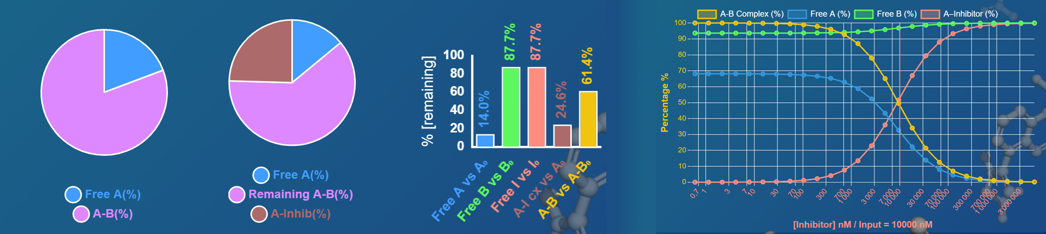
Additionally, important metrics are computed as percentages:
-
% of Protein A bound to Protein B:
\(\frac{[AB]}{[A]_{\text{tot}}}\times 100 = \frac{x}{[A]_{\text{tot}}}\times 100\)
-
% of Protein A bound to Inhibitor:
\(\frac{[AI]}{[A]_{\text{tot}}}\times 100 = \frac{y}{[A]_{\text{tot}}}\times 100\)
-
% of Inhibitor bound in complex:
\(\frac{[AI]}{[I]_{\text{tot}}}\times 100 = \frac{y}{[I]_{\text{tot}}}\times 100\)
-
% remaining AB (with I vs. no I):
\(\frac{[AB]_{\text{with inhib}}}{[AB]_{\text{no inhib}}}\times 100\)
Conclusion
The derivation starts from the fundamental principles of chemical kinetics and the mass-action law, proceeding through detailed algebraic
manipulation to obtain quadratic equations for simple binding and a set of coupled equations in the case of competitive inhibition.
The application of the Newton-Raphson method allows the solution to converge to the correct values. This comprehensive breakdown is
intended to enable any reader to understand every step from the theory to numerical execution in our solver.